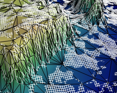
Canyon decimation example

Use the greedy-terrain-decimator to display a decimated terrain view.

This example illustrates decimating a terrain. We use the greedy-terrain-decimator to create a reduced mesh with an optimized grid that approximates the initial regular grid.

The initial grid is displayed in white, and the optimized grid is displayed in black, with the surface it creates. The initial grid can be seen disappearing as it goes under the surface of the approximated grid: although the decimated mesh follows closely the original, it is not exactly the same.

One can see that the reduction in number of polygons is huge: the white grid is much finer than the black grid. It is interesting to note that the decimated mesh follows closely the original mesh, including in number of polygons, in spots where the terrain changes most quickly.

This example uses the Grand Canyon topological radar data, from NASA.

The greedy-terrain-decimator is only useful to decimate a surface warped from 2D data. To decimated more general meshes, you can use the less-efficient decimate-pro filter (see Julia set decimation example).

Python source code: canyon_decimation.py

# Author: Gael Varoquaux <gael.varoquaux@normalesup.org>
# Copyright (c) 2008-2020, Enthought, Inc.
# License: BSD Style.

# Retrieve the grand Canyon topological data ###################################
# Original file:
#'ftp://e0srp01u.ecs.nasa.gov/srtm/version2/SRTM1/Region_04/N36W113.hgt.zip'
import os
if not os.path.exists('N36W113.hgt.zip'):
    # Download the data
    try:
        from urllib import urlopen
    except ImportError:
        from urllib.request import urlopen
    print('Downloading data, please wait (10M)')
    opener = urlopen(
    'https://s3.amazonaws.com/storage.enthought.com/www/sample_data/N36W113.hgt.zip'
        )
    open('N36W113.hgt.zip', 'wb').write(opener.read())

# Load the data (signed 2 byte integers, big endian) ###########################
import zipfile
import numpy as np

data = np.fromstring(zipfile.ZipFile('N36W113.hgt.zip').read('N36W113.hgt'),
                    '>i2')
data.shape = (3601, 3601)
data = data[200:400, 1200:1400]
data = data.astype(np.float32)

# Plot an interecting section ##################################################
from mayavi import mlab
mlab.figure(1, size=(450, 390))
mlab.clf()
data = mlab.pipeline.array2d_source(data)

# Use a greedy_terrain_decimation to created a decimated mesh
terrain = mlab.pipeline.greedy_terrain_decimation(data)
terrain.filter.error_measure = 'number_of_triangles'
terrain.filter.number_of_triangles = 5000
terrain.filter.compute_normals = True

# Plot it black the lines of the mesh
lines = mlab.pipeline.surface(terrain, color=(0, 0, 0),
                                      representation='wireframe')
# The terrain decimator has done the warping. We control the warping
# scale via the actor's scale.
lines.actor.actor.scale = [1, 1, 0.2]

# Display the surface itself.
surf = mlab.pipeline.surface(terrain, colormap='gist_earth',
                                      vmin=1450, vmax=1650)
surf.actor.actor.scale = [1, 1, 0.2]

# Display the original regular grid. This time we have to use a
# warp_scalar filter.
warp = mlab.pipeline.warp_scalar(data, warp_scale=0.2)
grid = mlab.pipeline.surface(warp, color=(1, 1, 1),
                                      representation='wireframe')

mlab.view(-17, 46, 143, [1.46, 8.46, 269.4])

mlab.show()