models Module¶

These classes are implementations of statistical models of annotations. They are available through the pyanno.models namespace, e.g.:

import pyanno.models
# create a new instance of model B, for 4 label classes and 6 annotators
model = pyanno.models.ModelB.create_initial_state(4, 6)

`modelB` Module¶

This module defines the class ModelB, a Bayesian generalization of the model proposed in (Dawid et al., 1979).

Reference:

Dawid, A. P. and A. M. Skene. 1979. Maximum likelihood estimation of observer error-rates using the EM algorithm. Applied Statistics, 28(1):20–28.

class pyanno.modelB.ModelB(nclasses, nannotators, pi, theta, alpha=None, beta=None, **traits)[source]¶

Bases: pyanno.abstract_model.AbstractModel

Bayesian generalization of the model proposed in (Dawid et al., 1979).

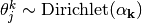
Model B is a hierarchical generative model over annotations. The model assumes the existence of “true” underlying labels for each item, which are drawn from a categorical distribution, $\pi$ . Annotators report this labels with some noise, depending on their accuracy, $\theta$ .

The model parameters are:

pi[k] is the probability of label k

theta[j,k,k’] is the probability that annotator j reports label k’ for an item whose real label is k, i.e. P( annotator j chooses k’ | real label = k)

The parameters themselves are random variables with hyperparameters

beta are the parameters of a Dirichlet distribution over pi

alpha[k,:] are the parameters of Dirichlet distributions over theta[j,k,:]

See the documentation for a more detailed description of the model.

References:

Dawid, A. P. and A. M. Skene. 1979. Maximum likelihood estimation of observer error-rates using the EM algorithm. Applied Statistics, 28(1):20–28.
Rzhetsky A., Shatkay, H., and Wilbur, W.J. (2009). “How to get the most from your curation effort”, PLoS Computational Biology, 5(5).

annotator_accuracy()[source]¶

Return the accuracy of each annotator.

Compute a summary of the a-priori accuracy of each annotator, i.e., P( annotator j is correct ). This can be computed from the parameters theta and pi, as

P( annotator j is correct ) = sum_k P( annotator j reports k | label is k ) P( label is k ) = sum_k theta[j,k,k] * pi[k]

Returns:	accuracy (ndarray, shape = (n_annotators, )) - accuracy[j] = P( annotator j is correct )

annotator_accuracy_samples(theta_samples, pi_samples)[source]¶

Return samples from the accuracy of each annotator.

Given samples from the posterior of accuracy parameters theta (see :method:`sample_posterior_over_accuracy`), compute samples from the posterior distribution of the annotator accuracy, i.e.,

P( annotator j is correct | annotations).

Returns:	accuracy (ndarray, shape = (n_annotators, )) - accuracy[j] = P( annotator j is correct )

static create_initial_state(nclasses, nannotators, alpha=None, beta=None)[source]¶

Factory method returning a model with random initial parameters.

It is often more convenient to use this factory method over the constructor, as one does not need to specify the initial model parameters.

The parameters theta and pi, controlling accuracy and prevalence, are initialized at random from the prior alpha and beta:

$\theta_j^k \sim \mathrm{Dirichlet}(\mathbf{\alpha_k})$

$\pi \sim \mathrm{Dirichlet}(\mathbf{\beta})$

If not defined, the prior parameters alpha ad beta are defined as described below.

Parameters:

nclasses (int) – Number of label classes
nannotators (int) – Number of annotators
alpha (ndarray) – Parameters of Dirichlet prior over annotator choices Default value is a band matrix that peaks at the correct annotation, with a value of 16 and decays to 1 with diverging classes. This prior is ideal for ordinal annotations.
beta (ndarray) – Parameters of Dirichlet prior over model categories Default value for beta[i] is 1.0 .

Returns:

model (ModelB) - Instance of ModelB

static default_alpha(nclasses)[source]¶

static default_beta(nclasses)[source]¶

generate_annotations(nitems)[source]¶

Generate a random annotation set from the model.

Sample a random set of annotations from the probability distribution defined the current model parameters:

Label classes are generated from the prior distribution, pi

Annotations are generated from the conditional distribution of annotations given classes, theta

Parameters:	nitems (int) – Number of items to sample
Returns:	annotations (ndarray, shape = (n_items, n_annotators)) - annotations[i,j] is the annotation of annotator j for item i

generate_annotations_from_labels(labels)[source]¶

Generate random annotations from the model, given labels

The method samples random annotations from the conditional probability distribution of annotations, $x_i^j$ given labels, $y_i$ :

$x_i^j \sim \mathrm{Categorical}(\mathbf{\theta_j^{y_i}})$

labels : ndarray, shape = (n_items,), dtype = int: Set of “true” labels

Returns:	annotations (ndarray, shape = (n_items, n_annotators)) - annotations[i,j] is the annotation of annotator j for item i

generate_labels(nitems)[source]¶: Generate random labels from the model.

infer_labels(annotations)[source]¶

Infer posterior distribution over label classes.

Compute the posterior distribution over label classes given observed annotations, $P( \mathbf{y} | \mathbf{x}, \theta, \omega)$ .

annotations : ndarray, shape = (n_items, n_annotators): annotations[i,j] is the annotation of annotator j for item i

Returns:	posterior (ndarray, shape = (n_items, n_classes)) - posterior[i,k] is the posterior probability of class k given the annotation observed in item i.

log_likelihood(annotations)[source]¶

Compute the log likelihood of a set of annotations given the model.

Returns log P(annotations | current model parameters).

annotations : ndarray, shape = (n_items, n_annotators): annotations[i,j] is the annotation of annotator j for item i

Returns:	log_lhood (float) - log likelihood of annotations

map(annotations, epsilon=1e-05, init_accuracy=0.6, max_epochs=1000)[source]¶

Computes maximum a posteriori (MAP) estimation of parameters.

Estimate the parameters theta and pi from a set of observed annotations using maximum a posteriori estimation.

annotations : ndarray, shape = (n_items, n_annotators): annotations[i,j] is the annotation of annotator j for item i
epsilon : float: The estimation is interrupted when the objective function has changed less than epsilon on average over the last 10 iterations
initial_accuracy : float: Initialize the accuracy parameters, theta to a set of distributions where theta[j,k,k’] = initial_accuracy if k==k’, and (1-initial_accuracy) / (n_classes - 1)
max_epoch : int: Interrupt the estimation after max_epoch iterations

mle(annotations, epsilon=1e-05, init_accuracy=0.6, max_epochs=1000)[source]¶

Computes maximum likelihood estimate (MLE) of parameters.

Estimate the parameters theta and pi from a set of observed annotations using maximum likelihood estimation.

annotations : ndarray, shape = (n_items, n_annotators): annotations[i,j] is the annotation of annotator j for item i
epsilon : float: The estimation is interrupted when the objective function has changed less than epsilon on average over the last 10 iterations
initial_accuracy : float: Initialize the accuracy parameters, theta to a set of distributions where theta[j,k,k’] = initial_accuracy if k==k’, and (1-initial_accuracy) / (n_classes - 1)
max_epoch : int: Interrupt the estimation after max_epoch iterations

sample_posterior_over_accuracy(annotations, nsamples, burn_in_samples=0, thin_samples=1, return_all_samples=True)[source]¶

Return samples from posterior distribution over theta given data.

Samples are drawn using Gibbs sampling, i.e., alternating between sampling from the conditional distribution of theta given the annotations and the label classes, and sampling from the conditional distribution of the classes given theta and the annotations.

This results in a fast-mixing sampler, and so the parameters controlling burn-in and thinning can be set to a small number of samples.

annotations : ndarray, shape = (n_items, n_annotators): annotations[i,j] is the annotation of annotator j for item i
nsamples : int: number of samples to draw from the posterior
burn_in_samples : int: Discard the first burn_in_samples during the initial burn-in phase, where the Monte Carlo chain converges to the posterior
thin_samples : int: Only return one every thin_samples samples in order to reduce the auto-correlation in the sampling chain. This is called “thinning” in MCMC parlance.
return_all_samples : bool: If True, return not only samples for the parameters theta, but also for the parameters pi, and the label classes, y.

Returns:	samples (ndarray, shape = (n_samples, n_annotators, nclasses, nclasses)) - samples[i,...] is one sample from the posterior distribution over the parameters theta

(theta, pi, labels) : tuple of ndarray: If the keyword argument return_all_samples is set to True, return a tuple with the samples for the parameters theta, the parameters pi, and the label classes, y

`modelBt` Module¶

This module defines model B-with-theta.

pyAnno includes another implementation of B-with-theta, pyanno.modelBt_loopdesign, which is optimized for a loop design where each item is annotated by 3 out of 8 annotators.

class pyanno.modelBt.ModelBt(nclasses, nannotators, gamma, theta, **traits)[source]¶

Bases: pyanno.abstract_model.AbstractModel

Implementation of Model B-with-theta from (Rzhetsky et al., 2009).

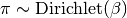
The model assumes the existence of “true” underlying labels for each item, which are drawn from a categorical distribution, gamma. Annotators report this labels with some noise, according to their accuracy, theta.

This model is closely related to ModelB, but, crucially, the noise distribution is described by a small number of parameters (one per annotator), which makes their estimation efficient and less sensitive to local optima.

The model parameters are:

gamma[k] is the probability of label k
theta[j] parametrizes the probability that annotator j reports label

k’ given ground truth, k. More specifically, P( annotator j chooses k’ | real label = k) is theta[j] for k’ = k, or (1 - theta[j]) / sum(theta) if `k’ != k `.

See the documentation for a more detailed description of the model.

For a version of this model optimized for the loop design described in (Rzhetsky et al., 2009), see ModelBtLoopDesign.

Reference

Rzhetsky A., Shatkay, H., and Wilbur, W.J. (2009). “How to get the most from your curation effort”, PLoS Computational Biology, 5(5).

static create_initial_state(nclasses, nannotators, gamma=None, theta=None)[source]¶

Factory method returning a model with random initial parameters.

It is often more convenient to use this factory method over the constructor, as one does not need to specify the initial model parameters.

The parameters theta and gamma, controlling accuracy and prevalence, are initialized at random as follows:

$\theta_j \sim \mathrm{Uniform}(0.6, 0.95)$

$\gamma \sim \mathrm{Dirichlet}(2.0)$

Parameters:

nclasses (int) – Number of label classes
nannotators (int) – Number of annotators
gamma (ndarray, shape = (n_classes, )) – gamma[k] is the prior probability of label class k
theta (ndarray, shape = (n_annotators, )) – theta[j] parametrizes the accuracy of annotator j. Specifically, P( annotator j chooses k’ | real label = k) is theta[j] for k’ = k, or (1 - theta[j]) / sum(theta) if `k’ != k `.

Returns:

model (ModelBt) - Instance of ModelBt

generate_annotations(nitems)[source]¶

Generate a random annotation set from the model.

Sample a random set of annotations from the probability distribution defined the current model parameters:

Label classes are generated from the prior distribution, pi

Annotations are generated from the conditional distribution of annotations given classes, parametrized by theta

Parameters:	nitems (int) – Number of items to sample
Returns:	annotations (ndarray, shape = (n_items, n_annotators)) - annotations[i,j] is the annotation of annotator j for item i

generate_annotations_from_labels(labels)[source]¶

Generate random annotations from the model, given labels

The method samples random annotations from the conditional probability distribution of annotations, $x_i^j$ given labels, $y_i$ .

labels : ndarray, shape = (n_items,), dtype = int: Set of “true” labels

Returns:	annotations (ndarray, shape = (n_items, n_annotators)) - annotations[i,j] is the annotation of annotator j for item i

generate_labels(nitems)[source]¶: Generate random labels from the model.

infer_labels(annotations)[source]¶

Infer posterior distribution over label classes.

Compute the posterior distribution over label classes given observed annotations, $P( \mathbf{y} | \mathbf{x}, \theta, \omega)$ .

annotations : ndarray, shape = (n_items, n_annotators): annotations[i,j] is the annotation of annotator j for item i

Returns:	posterior (ndarray, shape = (n_items, n_classes)) - posterior[i,k] is the posterior probability of class k given the annotation observed in item i.

log_likelihood(annotations)[source]¶

Compute the log likelihood of a set of annotations given the model.

Returns $\log P(\mathbf{x} | \gamma, \theta)$ , where $\mathbf{x}$ is the array of annotations.

annotations : ndarray, shape = (n_items, n_annotators): annotations[i,j] is the annotation of annotator j for item i

Returns:	log_lhood (float) - log likelihood of annotations

map(annotations, estimate_gamma=True)[source]¶

Computes maximum a posteriori (MAP) estimate of parameters.

Estimate the parameters theta and gamma from a set of observed annotations using maximum a posteriori estimation.

annotations : ndarray, shape = (n_items, n_annotators): annotations[i,j] is the annotation of annotator j for item i
estimate_gamma : bool: If True, the parameters gamma are estimated by the empirical class frequency. If False, gamma is left unchanged.

mle(annotations, estimate_gamma=True)[source]¶

Computes maximum likelihood estimate (MLE) of parameters.

Estimate the parameters theta and gamma from a set of observed annotations using maximum likelihood estimation.

annotations : ndarray, shape = (n_items, n_annotators): annotations[i,j] is the annotation of annotator j for item i
estimate_gamma : bool: If True, the parameters gamma are estimated by the empirical class frequency. If False, gamma is left unchanged.

sample_posterior_over_accuracy(annotations, nsamples, burn_in_samples=100, thin_samples=5, target_rejection_rate=0.3, rejection_rate_tolerance=0.2, step_optimization_nsamples=500, adjust_step_every=100)[source]¶

Return samples from posterior distribution over theta given data.

Samples are drawn using a variant of a Metropolis-Hasting Markov Chain Monte Carlo (MCMC) algorithm. Sampling proceeds in two phases:

step size estimation phase: first, the step size in the MCMC algorithm is adjusted to achieve a given rejection rate.

sampling phase: second, samples are collected using the step size from phase 1.

annotations : ndarray, shape = (n_items, n_annotators): annotations[i,j] is the annotation of annotator j for item i
nsamples : int: Number of samples to return (i.e., burn-in and thinning samples are not included)
burn_in_samples : int: Discard the first burn_in_samples during the initial burn-in phase, where the Monte Carlo chain converges to the posterior
thin_samples : int: Only return one every thin_samples samples in order to reduce the auto-correlation in the sampling chain. This is called “thinning” in MCMC parlance.
target_rejection_rate : float: target rejection rate for the step size estimation phase
rejection_rate_tolerance : float: the step size estimation phase is ended when the rejection rate for all parameters is within rejection_rate_tolerance from target_rejection_rate
step_optimization_nsamples : int: number of samples to draw in the step size estimation phase
adjust_step_every : int: number of samples after which the step size is adjusted during the step size estimation pahse

Returns:	samples (ndarray, shape = (n_samples, n_annotators)) - samples[i,:] is one sample from the posterior distribution over the parameters theta

`modelBt_loopdesign` Module¶

This module defines model B-with-theta, optimized for a loop design.

The implementation assumes that there are a total or 8 annotators. Each item is annotated by a triplet of annotators, according to the loop design described in Rzhetsky et al., 2009.

E.g., for 16 items the loop design looks like this (A indicates a label, * indicates a missing value):

A A A * * * * *
A A A * * * * *
* A A A * * * *
* A A A * * * *
* * A A A * * *
* * A A A * * *
* * * A A A * *
* * * A A A * *
* * * * A A A *
* * * * A A A *
* * * * * A A A
* * * * * A A A
A * * * * * A A
A * * * * * A A
A A * * * * * A
A A * * * * * A

class pyanno.modelBt_loopdesign.ModelBtLoopDesign(nclasses, gamma, theta, **traits)[source]¶

Bases: pyanno.abstract_model.AbstractModel

Implementation of Model B-with-theta from (Rzhetsky et al., 2009).

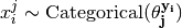
The model assumes the existence of “true” underlying labels for each item, which are drawn from a categorical distribution, gamma. Annotators report this labels with some noise.

This model is closely related to ModelB, but, crucially, the noise distribution is described by a small number of parameters (one per annotator), which makes their estimation efficient and less sensitive to local optima.

The model parameters are:

gamma[k] is the probability of label k
theta[j] parametrized the probability that annotator j reports label k’. More specifically, P( annotator j chooses k’ | real label = k) is theta[j] for k’ = k, or (1 - theta[j]) / sum(theta) if k’ != k .

This implementation is optimized for he loop design introduced in (Rzhetsky et al., 2009), which assumes that each item is annotated by 3 out of 8 annotators. For a more general implementation, see ModelBt

See the documentation for a more detailed description of the model.

Reference

Rzhetsky A., Shatkay, H., and Wilbur, W.J. (2009). “How to get the most from your curation effort”, PLoS Computational Biology, 5(5).

are_annotations_compatible(annotations)[source]¶: Check if the annotations are compatible with the models’ parameters.

static create_initial_state(nclasses, gamma=None, theta=None)[source]¶

Factory method returning a model with random initial parameters.

It is often more convenient to use this factory method over the constructor, as one does not need to specify the initial model parameters.

The parameters theta and gamma, controlling accuracy and prevalence, are initialized at random as follows:

$\theta_j \sim \mathrm{Uniform}(0.6, 0.95)$

$\gamma \sim \mathrm{Dirichlet}(2.0)$

Parameters:	nclasses (int) – number of categories gamma (nparray) – An array of floats with size that holds the probability of each annotation value. Default is None theta (nparray) – An array of floats that the parameters of P( v_i \| psi ) (one for each annotator)
Returns:	model (`ModelBtLoopDesign`) - Instance of ModelBtLoopDesign

generate_annotations(nitems)[source]¶

Generate a random annotation set from the model.

Sample a random set of annotations from the probability distribution defined the current model parameters:

Label classes are generated from the prior distribution, pi

Annotations are generated from the conditional distribution of annotations given classes, parametrized by theta

Parameters:	nitems (int) – Number of items to sample
Returns:	annotations (ndarray, shape = (n_items, n_annotators)) - annotations[i,j] is the annotation of annotator j for item i

generate_annotations_from_labels(labels)[source]¶

Generate random annotations from the model, given labels

The method samples random annotations from the conditional probability distribution of annotations, $x_i^j$ given labels, $y_i$ .

labels : ndarray, shape = (n_items,), dtype = int: Set of “true” labels

Returns:	annotations (ndarray, shape = (n_items, n_annotators)) - annotations[i,j] is the annotation of annotator j for item i

generate_labels(nitems)[source]¶: Generate random labels from the model.

infer_labels(annotations)[source]¶

Infer posterior distribution over label classes.

Compute the posterior distribution over label classes given observed annotations, $P( \mathbf{y} | \mathbf{x}, \theta, \omega)$ .

annotations : ndarray, shape = (n_items, n_annotators): annotations[i,j] is the annotation of annotator j for item i

Returns:	posterior (ndarray, shape = (n_items, n_classes)) - posterior[i,k] is the posterior probability of class k given the annotation observed in item i.

log_likelihood(annotations)[source]¶

Compute the log likelihood of a set of annotations given the model.

Returns $\log P(\mathbf{x} | \gamma, \theta)$ , where $\mathbf{x}$ is the array of annotations.

annotations : ndarray, shape = (n_items, n_annotators): annotations[i,j] is the annotation of annotator j for item i

Returns:	log_lhood (float) - log likelihood of annotations

map(annotations, estimate_gamma=True)[source]¶

Computes maximum a posteriori (MAP) estimate of parameters.

Estimate the parameters theta and gamma from a set of observed annotations using maximum a posteriori estimation.

annotations : ndarray, shape = (n_items, n_annotators): annotations[i,j] is the annotation of annotator j for item i
estimate_gamma : bool: If True, the parameters gamma are estimated by the empirical class frequency. If False, gamma is left unchanged.

mle(annotations, estimate_gamma=True)[source]¶

Computes maximum likelihood estimate (MLE) of parameters.

Estimate the parameters theta and gamma from a set of observed annotations using maximum likelihood estimation.

annotations : ndarray, shape = (n_items, n_annotators): annotations[i,j] is the annotation of annotator j for item i
estimate_gamma : bool: If True, the parameters gamma are estimated by the empirical class frequency. If False, gamma is left unchanged.

sample_posterior_over_accuracy(annotations, nsamples, burn_in_samples=100, thin_samples=5, target_rejection_rate=0.3, rejection_rate_tolerance=0.2, step_optimization_nsamples=500, adjust_step_every=100)[source]¶

Return samples from posterior distribution over theta given data.

Samples are drawn using a variant of a Metropolis-Hasting Markov Chain Monte Carlo (MCMC) algorithm. Sampling proceeds in two phases:

step size estimation phase: first, the step size in the MCMC algorithm is adjusted to achieve a given rejection rate.

sampling phase: second, samples are collected using the step size from phase 1.

annotations : ndarray, shape = (n_items, n_annotators): annotations[i,j] is the annotation of annotator j for item i
nsamples : int: Number of samples to return (i.e., burn-in and thinning samples are not included)
burn_in_samples : int: Discard the first burn_in_samples during the initial burn-in phase, where the Monte Carlo chain converges to the posterior
thin_samples : int: Only return one every thin_samples samples in order to reduce the auto-correlation in the sampling chain. This is called “thinning” in MCMC parlance.
target_rejection_rate : float: target rejection rate for the step size estimation phase
rejection_rate_tolerance : float: the step size estimation phase is ended when the rejection rate for all parameters is within rejection_rate_tolerance from target_rejection_rate
step_optimization_nsamples : int: number of samples to draw in the step size estimation phase
adjust_step_every : int: number of samples after which the step size is adjusted during the step size estimation pahse

Returns:	samples (ndarray, shape = (n_samples, n_annotators)) - samples[i,:] is one sample from the posterior distribution over the parameters theta

`modelA` Module¶

This module defines the class ModelA, an implementation of model A from Rzhetsky et al., 2009.

The implementation assumes that there are a total or 8 annotators. Each item is annotated by a triplet of annotators, according to the loop design described in Rzhetsky et al., 2009.

E.g., for 16 items the loop design looks like this (A indicates a label, * indicates a missing value):

A A A * * * * *
A A A * * * * *
* A A A * * * *
* A A A * * * *
* * A A A * * *
* * A A A * * *
* * * A A A * *
* * * A A A * *
* * * * A A A *
* * * * A A A *
* * * * * A A A
* * * * * A A A
A * * * * * A A
A * * * * * A A
A A * * * * * A
A A * * * * * A

Reference

Rzhetsky A., Shatkay, H., and Wilbur, W.J. (2009). “How to get the most from your curation effort”, PLoS Computational Biology, 5(5).

class pyanno.modelA.ModelA(nclasses, theta, omega, **traits)[source]¶

Bases: pyanno.abstract_model.AbstractModel

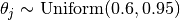
Implementation of Model A from (Rzhetsky et al., 2009).

The model defines a probability distribution over data annotations in which each item is annotated by three users. The distributions is described according to a three-steps generative model:

1. First, the model independently generates correctness values for the triplet of annotators (e.g., CCI where C=correct, I=incorrect)

2. Second, the model generates an agreement pattern compatible with the correctness values (e.g., CII is compatible with the agreement patterns ‘abb’ and ‘abc’, where different letters correspond to different annotations

3. Finally, the model generates actual observations compatible with the agreement patterns

The model has two main sets of parameters:

theta[j] is the probability that annotator j is correct

omega[k] is the probability of observing an annotation of class k over all items and annotators

At the moment the implementation of the model assumes 1) a total of 8 annotators, and 2) each item is annotated by exactly 3 annotators.

See the documentation for a more detailed description of the model.

Reference

Rzhetsky A., Shatkay, H., and Wilbur, W.J. (2009). “How to get the most from your curation effort”, PLoS Computational Biology, 5(5).

are_annotations_compatible(annotations)[source]¶: Check if the annotations are compatible with the models’ parameters.

static create_initial_state(nclasses, theta=None, omega=None)[source]¶

Factory method to create a new model.

It is often more convenient to use this factory method over the constructor, as one does not need to specify the initial model parameters.

If not specified, the parameters theta are drawn from a uniform distribution between 0.6 and 0.95 . The parameters omega are drawn from a Dirichlet distribution with parameters 2.0 :

$\theta_j \sim \mathrm{Uniform}(0.6, 0.95)$

$\omega_k \sim \mathrm{Dirichlet}(2.0)$

Parameters:	nclasses (int) – number of possible annotation classes theta (ndarray, shape = (n_annotators, )) – theta[j] is the probability of annotator j being correct omega (ndarray, shape = (n_classes, )) – omega[k] is the probability of observing a label of class k

generate_annotations(nitems)[source]¶

Generate random annotations from the model.

The method samples random annotations from the probability distribution defined by the model parameters:

generate correct/incorrect labels for the three annotators, according to the parameters theta

generate agreement patterns (which annotator agrees which whom) given the correctness information and the parameters alpha

generate the annotations given the agreement patterns and the parameters omega

Note that, according to the model’s definition, only three annotators per item return an annotation. Non-observed annotations have the standard value of MISSING_VALUE.

Parameters:	nitems (int) – number of annotations to draw from the model
Returns:	annotations (ndarray, shape = (n_items, n_annotators)) - annotations[i,j] is the annotation of annotator j for item i

infer_labels(annotations)[source]¶

Infer posterior distribution over label classes.

Compute the posterior distribution over label classes given observed annotations, $P( \mathbf{y} | \mathbf{x}, \theta, \omega)$ .

Parameters:	annotations (ndarray, shape = (n_items, n_annotators)) – annotations[i,j] is the annotation of annotator j for item i
Returns:	posterior (ndarray, shape = (n_items, n_classes)) - posterior[i,k] is the posterior probability of class k given the annotation observed in item i.

log_likelihood(annotations)[source]¶

Compute the log likelihood of a set of annotations given the model.

Returns $\log P(\mathbf{x} | \omega, \theta)$ , where $\mathbf{x}$ is the array of annotations.

Parameters:	annotations (ndarray, shape = (n_items, n_annotators)) – annotations[i,j] is the annotation of annotator j for item i
Returns:	log_lhood (float) - log likelihood of annotations

map(annotations, estimate_omega=True)[source]¶

Computes maximum a posteriori (MAP) estimate of parameters.

Estimate the parameters theta and omega from a set of observed annotations using maximum a posteriori estimation.

Parameters:	annotations (ndarray, shape = (n_items, n_annotators)) – annotations[i,j] is the annotation of annotator j for item i estimate_omega (bool) – If True, the parameters `omega` are estimated by the empirical class frequency. If False, `omega` is left unchanged.

mle(annotations, estimate_omega=True)[source]¶

Computes maximum likelihood estimate (MLE) of parameters.

Estimate the parameters theta and omega from a set of observed annotations using maximum likelihood estimation.

Parameters:	annotations (ndarray, shape = (n_items, n_annotators)) – annotations[i,j] is the annotation of annotator j for item i estimate_omega (bool) – If True, the parameters `omega` are estimated by the empirical class frequency. If False, `omega` is left unchanged.

sample_posterior_over_accuracy(annotations, nsamples, burn_in_samples=100, thin_samples=5, target_rejection_rate=0.3, rejection_rate_tolerance=0.2, step_optimization_nsamples=500, adjust_step_every=100)[source]¶

Return samples from posterior distribution over theta given data.

Samples are drawn using a variant of a Metropolis-Hasting Markov Chain Monte Carlo (MCMC) algorithm. Sampling proceeds in two phases:

step size estimation phase: first, the step size in the MCMC algorithm is adjusted to achieve a given rejection rate.

sampling phase: second, samples are collected using the step size from phase 1.

Parameters:

annotations (ndarray, shape = (n_items, n_annotators)) – annotations[i,j] is the annotation of annotator j for item i
nsamples (int) – number of samples to draw from the posterior
burn_in_samples (int) – Discard the first burn_in_samples during the initial burn-in phase, where the Monte Carlo chain converges to the posterior
thin_samples (int) – Only return one every thin_samples samples in order to reduce the auto-correlation in the sampling chain. This is called “thinning” in MCMC parlance.
target_rejection_rate (float) – target rejection rate for the step size estimation phase
rejection_rate_tolerance (float) – the step size estimation phase is ended when the rejection rate for all parameters is within rejection_rate_tolerance from target_rejection_rate
step_optimization_nsamples (int) – number of samples to draw in the step size estimation phase
adjust_step_every (int) – number of samples after which the step size is adjusted during the step size estimation pahse

Returns:

samples (ndarray, shape = (n_samples, n_annotators)) - samples[i,:] is one sample from the posterior distribution over the parameters theta

models Module¶

`modelB` Module¶

`modelBt` Module¶

`modelBt_loopdesign` Module¶

`modelA` Module¶

Table Of Contents

Previous topic

Next topic

This Page

Navigation

models Module¶

modelB Module¶

modelBt Module¶

modelBt_loopdesign Module¶

modelA Module¶

Table Of Contents

Previous topic

Next topic

This Page

Quick search

Navigation

`modelB` Module¶

`modelBt` Module¶

`modelBt_loopdesign` Module¶

`modelA` Module¶