Organisation of Mayavi visualizations: the pipeline
Anatomy of a Mayavi pipeline
Layout of a pipeline
The top node of a Mayavi pipeline is called the Engine. It is responsible of the creation and destruction of the scenes. It is not displayed in the pipeline view.
Below the Engine, you find Scenes.
Each Scene has a set of data Sources: they expose the data to visualize to Mayavi.
Filters can be applied to the Sources to transform the data they wrap.
A Module Manager controls the colors used to represent the scalar or vector data. It is represented in the pipeline view as the node called Colors and legends.
Visualization Modules finally display a reprensation of the data in the Scene, such as a surface, or lines.
The link between different Mayavi entry points
Every visualization created in Mayavi is constructed with a pipeline, although the construction of the pipeline may be hidden from the user:
The easiest way to make a Mayavi visualization is to create a pipeline via the user interface, as, for instance, exposed in the Parametric surfaces examples.
The mlab 3d plotting functions, create full piplelines, comprising sources, modules, and possibly filters, to visualize numpy arrays. Displaying the pipeline view is the easiest way to understand what pipeline was built.
Pipelines can also be built node-by-node with mlab, using the mlab.pipeline functions. The name of the functions to call can simply be deduced from the names of the pipeline nodes as they appear in the pipeline view.
The objects composing a pipeline can be instantiated and added to the pipeline manually, as exposed further below.
A pipeline example examined
Let us study the pipeline created by the mlab.plot3d function to represent lines:
import numpy as np
phi = np.linspace(0., 2*np.pi, 1000)
x   = np.cos(6*phi)*(1 + .5*np.cos(11*phi))
y   = np.sin(6*phi)*(1 + .5*np.cos(11*phi))
z   = .5*np.sin(11*phi)

from mayavi import mlab
surface = mlab.plot3d(x, y, z, np.sin(6*phi), tube_radius=0.025, colormap='Spectral', opacity=.5)
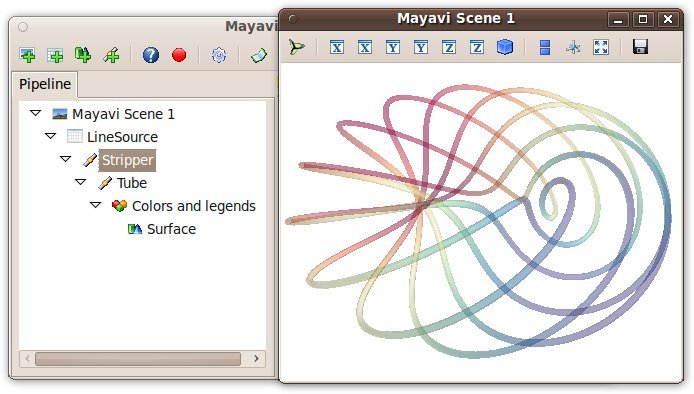
The mlab.plot3d function first creates a source made of points connected by lines. Then it applies the Stripper filter, which transforms this succession of lines in a ‘strip’. Second, a Tube filter is applied: from the ‘strip’ it creates tubes with a given radius. Finally, the Surface module is applied to display the surface of the tubes. The surface object returned by the mlab.plot3d function is that final Surface module.
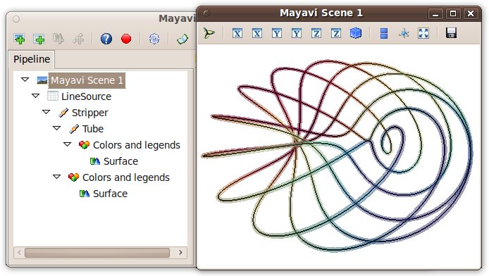
Let us have a look at the data in the pipeline before the tube filter was applied. First we retrive the Stripper filter:
stripper = surface.parent.parent.parent
Then we apply on it a Surface module to represent the strip:
lines = mlab.pipeline.surface(stripper, color=(0, 0, 0))
All the properties of the different steps can be adjusted in the pipeline view. In addition, they correspond to attributes on the various objects:
>>> tubes = surface.parent.parent
>>> tubes.filter.radius
0.025000000000000001
The names in the dialogs of the various properties gives hints to which attributes in the objects they correspond to. However, it can be fairly challenging to find this correspondance. We suggest to use the record feature for this purpose.