Assembling pipelines with mlab
The plotting functions reviewed above explore only a small fraction of the visualization possibilities of Mayavi. The full power of Mayavi can only be unleashed through the control of the pipeline itself. As described in the An overview of Mayavi section, a visualization in Mayavi is created by loading the data in Mayavi with data source object, optionally transforming the data through Filters, and visualizing it with Modules. The mlab functions build complex pipelines for you in one function, making the right choice of sources, filters, and modules, but they cannot explore all the possible combinations.
Mlab provides a sub-module pipeline which contains functions to populate the pipeline easily from scripts. This module is accessible in mlab: mlab.pipeline, or can be imported from mayavi.tools.pipeline.
When using an mlab plotting function, a pipeline is created: first a
source is created from numpy arrays, then modules, and possibly
filters, are added. The resulting pipeline can be seen for instance with
the mlab.show_pipeline command. This information can be used to create
the very same pipeline directly using the pipeline scripting module, as
the names of the functions required to create each step of the pipeline
are directly linked to the default names of the objects created by mlab
on the pipeline. As an example, let us create a visualization using
surf():
import numpy as np
a = np.random.random((4, 4))
from mayavi import mlab
mlab.surf(a)
mlab.show_pipeline()
The following pipeline is created:
Array2DSource
    \__ WarpScalar
            \__ PolyDataNormals
                    \__ Colors and legends
                            \__ Surface
The same pipeline can be created using the following code:
src = mlab.pipeline.array2d_source(a)
warp = mlab.pipeline.warp_scalar(src)
normals = mlab.pipeline.poly_data_normals(warp)
surf = mlab.pipeline.surface(normals)
Data sources
The mlab.pipeline module contains functions for creating various data sources from arrays. They are fully documented in details in the Mlab pipeline-control reference. We give a small summary of the possibilities here.
Mayavi distinguishes sources with scalar data, and sources with vector data, but more important, it has different functions to create sets of unconnected points, with data attached to them, or connected data points describing continuously varying quantities that can be interpolated between data points, often called fields in physics or engineering.
- Unconnected sources:
scalar_scatter()(creates a PolyData)
vector_scatter()(creates an PolyData)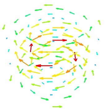
- implicitly-connected sources:
scalar_field()(creates an ImageData)
vector_field()(creates an ImageData)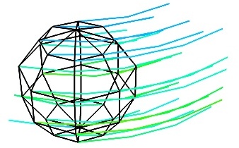
array2d_source()(creates an ImageData)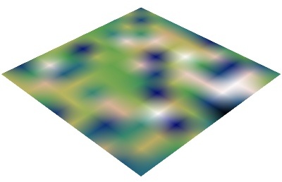
- Explicitly-connected sources:
line_source()(creates an PolyData)
triangular_mesh_source()(creates an PolyData)
All the mlab.pipline source factories are functions that take numpy arrays and return the Mayavi source object that was added to the pipeline. However, the implicitly-connected sources require well-shaped arrays as arguments: the data is supposed to lie on a regular, orthogonal, grid of the same shape as the shape of the input array, in other words, the array describes an image, possibly 3 dimensional.
Note
More complicated data structures can be created, such as irregular grids or non-orthogonal grid. See the section on data structures.
Modules and filters
For each Mayavi module or filter (see Modules and Filters), there is a corresponding mlab.pipeline function. The name of this function is created by replacing the alternating capitals in the module or filter name by underscores. Thus ScalarCutPlane corresponds to scalar_cut_plane.
In general, the mlab.pipeline module and filter factory functions simply create and connect the corresponding object. However they can also contain addition logic, exposed as keyword arguments. For instance they allow to set up easily a colormap, or to specify the color of the module, when relevant. In accordance with the goal of the mlab interface to make frequent operations simple, they use the keyword arguments to choose the properties of the created object to suit the requirements. It can be thus easier to use the keyword arguments, when available, than to set the attributes of the objects created. For more information, please check out the docstrings. Full, detailed, usage examples are given in the next subsection.