Protein example
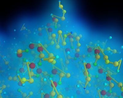
Visualize a protein graph structure downloaded from the protein database in standard pdb format.
We parse the pdb file, but extract only a very small amount of information: the type of atoms, their positions, and the links between them.
Most of the complexity of this example comes from the code turning the PDB information into a list of 3D positions, with associated scalar and connection information.
We assign a scalar value for the atoms to differenciate the different types of atoms, but it does not correspond to the atomic mass. The size and the color of the atom on the visualization is therefore not chemicaly-significant.
The atoms are plotted using mlab.points3d, and connections between atoms are added to the dataset, and visualized using a surface module.
The graph is created by adding connection information to points. For this, each point is designated by its number (in the order of the array passed to mlab.points3d), and the connection array, made of pairs of these numbers, is constructed. There is some slightly tedious data manipulation to go from the named-node graph representation as stored in the pdb file, to the index-based connection pairs. A similar technique to plot the graph is done in the Flight graph example. Another example of graph plotting, showing a different technique to plot the graph, can be seen on Delaunay graph example.
To visualize the local atomic density, we use a gaussian splatter filter that builds a kernel density estimation of the continuous density field: each point is convoluted by a Gaussian kernel, and the sum of these Gaussians form the resulting density field. We visualize this field using volume rendering.
Reference for the pdb file standard: http://mmcif.pdb.org/dictionaries/pdb-correspondence/pdb2mmcif.html

Python source code: protein.py
# Author: Gael Varoquaux <gael.varoquaux@normalesup.org>
# Copyright (c) 2008-2020, Enthought, Inc.
# License: BSD Style.

# The pdb code for the protein.
protein_code = '2q09'

# Retrieve the file from the protein database #################################
import os
if not os.path.exists('pdb%s.ent.gz' % protein_code):
    # Download the data
    try:
        from urllib import urlopen
    except ImportError:
        from urllib.request import urlopen
    print('Downloading protein data, please wait')
    opener = urlopen(
      'ftp://ftp.wwpdb.org/pub/pdb/data/structures/divided/pdb/q0/pdb%s.ent.gz'
      % protein_code)
    open('pdb%s.ent.gz' % protein_code, 'wb').write(opener.read())

# Parse the pdb file ##########################################################
import gzip
infile = gzip.GzipFile('pdb%s.ent.gz' % protein_code, 'rb')

# A graph represented by a dictionary associating nodes with keys
# (numbers), and edges (pairs of node keys).
nodes = dict()
edges = list()
atoms = set()

# Build the graph from the PDB information
last_atom_label = None
last_chain_label = None
for line in infile:
    line = line.split()
    if line[0] in ('ATOM', 'HETATM'):
        nodes[line[1]] = (line[2], line[6], line[7], line[8])
        atoms.add(line[2])
        chain_label = line[5]
        if chain_label == last_chain_label:
            edges.append((line[1], last_atom_label))
        last_atom_label = line[1]
        last_chain_label = chain_label
    elif line[0] == 'CONECT':
        for start, stop in zip(line[1:-1], line[2:]):
            edges.append((start, stop))

atoms = list(atoms)
atoms.sort()
atoms = dict(zip(atoms, range(len(atoms))))

# Turn the graph into 3D positions, and a connection list.
labels = dict()

x = list()
y = list()
z = list()
scalars = list()

for index, label in enumerate(nodes):
    labels[label] = index
    this_scalar, this_x, this_y, this_z = nodes[label]
    scalars.append(atoms[this_scalar])
    x.append(float(this_x))
    y.append(float(this_y))
    z.append(float(this_z))

connections = list()

for start, stop in edges:
    connections.append((labels[start], labels[stop]))

import numpy as np
x = np.array(x)
y = np.array(y)
z = np.array(z)
scalars = np.array(scalars)

# Visualize the data ##########################################################
from mayavi import mlab
mlab.figure(1, bgcolor=(0, 0, 0))
mlab.clf()

pts = mlab.points3d(x, y, z, 1.5 * scalars.max() - scalars,
                                    scale_factor=0.015, resolution=10)
pts.mlab_source.dataset.lines = np.array(connections)

# Use a tube fiter to plot tubes on the link, varying the radius with the
# scalar value
tube = mlab.pipeline.tube(pts, tube_radius=0.15)
tube.filter.radius_factor = 1.
tube.filter.vary_radius = 'vary_radius_by_scalar'
mlab.pipeline.surface(tube, color=(0.8, 0.8, 0))

# Visualize the local atomic density
mlab.pipeline.volume(mlab.pipeline.gaussian_splatter(pts))

mlab.view(49, 31.5, 52.8, (4.2, 37.3, 20.6))

mlab.show()
