Atomic orbital example
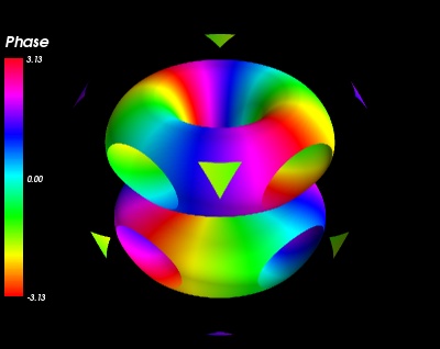
An example showing the norm and phase of an atomic orbital: isosurfaces of the norm, with colors displaying the phase.
This example shows how you can apply a filter on one data set, and dislay a second data set on the output of the filter. Here we use the contour filter to extract isosurfaces of the norm of a complex field, and we display the phase of the field with the colormap.
The field we choose to plot is a simplified version of the 3P_y atomic orbital for hydrogen-like atoms.
The first step is to create a data source with two scalar datasets. The second step is to apply filters and modules, using the ‘set_active_attribute’ filter to select on which data these apply.
Creating a data source with two scalar datasets is actually slightly tricky, as it requires some understanding of the layout of the datasets in TVTK. The reader is referred to Data representation in Mayavi for more details.

Python source code: atomic_orbital.py
# Author: Gael Varoquaux <gael.varoquaux@normalesup.org>
# Copyright (c) 2008, Enthought, Inc.
# License: BSD Style.

# Create the data ############################################################
import numpy as np

x, y, z = np.ogrid[- .5:.5:200j, - .5:.5:200j, - .5:.5:200j]
r = np.sqrt(x ** 2 + y ** 2 + z ** 2)


# Generalized Laguerre polynomial (3, 2)
L = - r ** 3 / 6 + 5. / 2 * r ** 2 - 10 * r + 6

# Spherical harmonic (3, 2)
Y = (x + y * 1j) ** 2 * z / r ** 3

Phi = L * Y * np.exp(- r) * r ** 2

# Plot it ####################################################################
from mayavi import mlab
mlab.figure(1, fgcolor=(1, 1, 1), bgcolor=(0, 0, 0))
# We create a scalar field with the module of Phi as the scalar
src = mlab.pipeline.scalar_field(np.abs(Phi))

# And we add the phase of Phi as an additional array
# This is a tricky part: the layout of the new array needs to be the same
# as the existing dataset, and no checks are performed. The shape needs
# to be the same, and so should the data. Failure to do so can result in
# segfaults.
src.image_data.point_data.add_array(np.angle(Phi).T.ravel())
# We need to give a name to our new dataset.
src.image_data.point_data.get_array(1).name = 'angle'
# Make sure that the dataset is up to date with the different arrays:
src.update()

# We select the 'scalar' attribute, ie the norm of Phi
src2 = mlab.pipeline.set_active_attribute(src,
                                    point_scalars='scalar')

# Cut isosurfaces of the norm
contour = mlab.pipeline.contour(src2)

# Now we select the 'angle' attribute, ie the phase of Phi
contour2 = mlab.pipeline.set_active_attribute(contour,
                                    point_scalars='angle')

# And we display the surface. The colormap is the current attribute: the phase.
mlab.pipeline.surface(contour2, colormap='hsv')

mlab.colorbar(title='Phase', orientation='vertical', nb_labels=3)

mlab.show()
