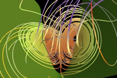
Lorenz example

An example displaying the trajectories for the Lorenz system of equations along with the z-nullcline.

The vector field of the Lorenz system flow is integrated to display trajectories using mlab’s flow function: mayavi.mlab.flow().

The z-nullcline is plotted by extracting the z component of the vector field data source with the ExtractVectorComponent filter, and applying an IsoSurface module on this scalar component.

Python source code: lorenz.py

# Author: Prabhu Ramachandran <prabhu@aero.iitb.ac.in>
# Copyright (c) 2008-2020, Enthought, Inc.
# License: BSD Style.

import numpy
from mayavi import mlab


def lorenz(x, y, z, s=10., r=28., b=8. / 3.):
    """The Lorenz system."""
    u = s * (y - x)
    v = r * x - y - x * z
    w = x * y - b * z
    return u, v, w

# Sample the space in an interesting region.
x, y, z = numpy.mgrid[-50:50:100j, -50:50:100j, -10:60:70j]
u, v, w = lorenz(x, y, z)
fig = mlab.figure(size=(400, 300), bgcolor=(0, 0, 0))

# Plot the flow of trajectories with suitable parameters.
f = mlab.flow(x, y, z, u, v, w, line_width=3, colormap='Paired')
f.module_manager.scalar_lut_manager.reverse_lut = True
f.stream_tracer.integration_direction = 'both'
f.stream_tracer.maximum_propagation = 200
# Uncomment the following line if you want to hide the seed:
#f.seed.widget.enabled = False

# Extract the z-velocity from the vectors and plot the 0 level set
# hence producing the z-nullcline.
src = f.mlab_source.m_data
e = mlab.pipeline.extract_vector_components(src)
e.component = 'z-component'
zc = mlab.pipeline.iso_surface(e, opacity=0.5, contours=[0, ],
            color=(0.6, 1, 0.2))
# When using transparency, hiding 'backface' triangles often gives better
# results
zc.actor.property.backface_culling = True

# A nice view of the plot.
mlab.view(140, 120, 113, [0.65, 1.5, 27])
mlab.show()