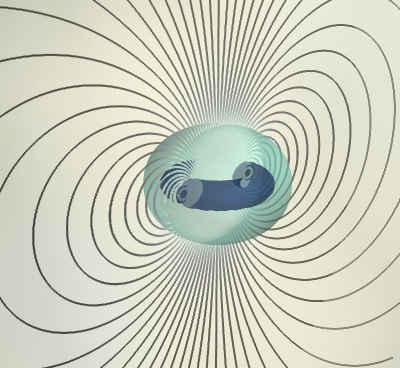
Magnetic field lines example

This example uses the streamline module to display field lines of a magnetic dipole (a current loop).

This example requires scipy.

The magnetic field from an arbitrary current loop is calculated from eqns (1) and (2) in Phys Rev A Vol. 35, N 4, pp. 1535-1546; 1987.

To get a prettier result, we use a fairly large grid to sample the field. As a consequence, we need to clear temporary arrays as soon as possible.

For a more thorough example of magnetic field calculation and visualization with Mayavi and scipy, see Magnetic field example.

Python source code: magnetic_field_lines.py

# Author: Gael Varoquaux <gael.varoquaux@normalesup.org>
# Copyright (c) 2007, Enthought, Inc.
# License: BSD Style.

import numpy as np
from scipy import special

#### Calculate the field ####################################################
radius = 1  # Radius of the coils

x, y, z = [e.astype(np.float32) for e in
            np.ogrid[-10:10:150j, -10:10:150j, -10:10:150j]]

# express the coordinates in polar form
rho = np.sqrt(x ** 2 + y ** 2)
x_proj = x / rho
y_proj = y / rho
# Free memory early
del x, y

E = special.ellipe((4 * radius * rho) / ((radius + rho) ** 2 + z ** 2))
K = special.ellipk((4 * radius * rho) / ((radius + rho) ** 2 + z ** 2))
Bz = 1 / np.sqrt((radius + rho) ** 2 + z ** 2) * (
                K
                + E * (radius ** 2 - rho ** 2 - z ** 2) /
                    ((radius - rho) ** 2 + z ** 2)
            )
Brho = z / (rho * np.sqrt((radius + rho) ** 2 + z ** 2)) * (
                - K
                + E * (radius ** 2 + rho ** 2 + z ** 2) /
                    ((radius - rho) ** 2 + z ** 2)
            )
del E, K, z, rho
# On the axis of the coil we get a divided by zero. This returns a
# NaN, where the field is actually zero :
Brho[np.isnan(Brho)] = 0

Bx, By = x_proj * Brho, y_proj * Brho

del x_proj, y_proj, Brho

#### Visualize the field ####################################################
from mayavi import mlab
fig = mlab.figure(1, size=(400, 400), bgcolor=(1, 1, 1), fgcolor=(0, 0, 0))

field = mlab.pipeline.vector_field(Bx, By, Bz)
# Unfortunately, the above call makes a copy of the arrays, so we delete
# this copy to free memory.
del Bx, By, Bz

magnitude = mlab.pipeline.extract_vector_norm(field)
contours = mlab.pipeline.iso_surface(magnitude,
                                        contours=[0.01, 0.8, 3.8, ],
                                        transparent=True,
                                        opacity=0.4,
                                        colormap='YlGnBu',
                                        vmin=0, vmax=2)


field_lines = mlab.pipeline.streamline(magnitude, seedtype='line',
                                        integration_direction='both',
                                        colormap='bone',
                                        vmin=0, vmax=1)

# Tweak a bit the streamline.
field_lines.stream_tracer.maximum_propagation = 100.
field_lines.seed.widget.point1 = [69, 75.5, 75.5]
field_lines.seed.widget.point2 = [82, 75.5, 75.5]
field_lines.seed.widget.resolution = 50
field_lines.seed.widget.enabled = False

mlab.view(42, 73, 104, [79,  75,  76])

mlab.show()